LoC
This project is maintained by clarkdatalabs
Choosing MARC Fields
The library of congress organizes their record metadata following the MARC (MAchine Readable Cataloging) standard. There are many different Library of Congress record metadata fields available, but I wanted to do a project with a spatial component, so I settled on manipulations of the following:
- 260c: Date of publication, distribution, etc.: Our main temporal variable.
- 650a: Subject Added Entry; Topical term or geographic name entry element: We will geocode strings about subject location, which will become our main spatial variable.
- 050a: Classification number: Letters at the beginning of classification numbers indicate subject area, which we may explore in the future.
Ok, so I've chosen what I want to work with - but how do you go about getting records and just these fields, in a form that is ready for visualizing?
Parsing XML Record Files
I restricted myself to just book records, which are available for download in 41 separate compressed .XML files. Each uncompressed XML file is more than 500 megabytes - this is a lot of data! With files this large, loading them entirely into memory as you would with standard XML parsing methods becomes impractical (especially on my laptop). Instead, we have to use iterative parsing to step through the XML, node by node, without loading the entire tree structure into memory.
The Python package lxml provides tools for doing exactly this, namely an implementation of the etree.iterparse() function. There are some examples of this on the lxml site, but I found this overall explanation of iterative XML parsing to be really helpful as well. We will want to iterate through “record” items. Then for each one, find all subfields with the tags corresponding to the chosen MARC fields.
At this stage, we have some initial cleaning that is also necessary. We might expect 260c – Date of publication, distribution, etc. to be a simple integer year telling us the year of publication. No such luck:
<datafield tag="260" ind1=" " ind2=" ">
	<subfield code="a">New York city,</subfield>
	<subfield code="b">Dau publishing co.,</subfield>
	<subfield code="c">c1899.</subfield>
We can roughly extract years from these strings by taking the first instance of exactly four consecutive digits using the regular expression function:
re.findall(r'(?<!\d)\d{4}(?!\d)',date_string)Similarly we might want to strip some of the punctuation out of the subject location strings with the translate method:
.translate({ord(c): None for c in '[];:?,.'})Storing the Parsed Fields
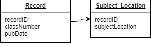
Great, we can parse the records, but we’re going to need to save them somewhere if we hope to use them in our visualization. Each record may have several subject locations, so our data structure needs to handle a one to many relationship. Given that we may be working with several million records that have these fields populated, we’ll use a SQLite database with a couple tables to start:
Once you have installed SQLite, the sqlite3 python package makes it easy to create and interact with our SQLite database from our Python script. This thorough guide to using sqlite3 might be really helpful, especially if you’re just getting started with SQLite like me.
Geocoding Subject Locations
The big challenge of this project is turning the subjectLocation strings into actual locations that can be mapped. Here’s an example of some of the strings stored in the Subject_Location table:
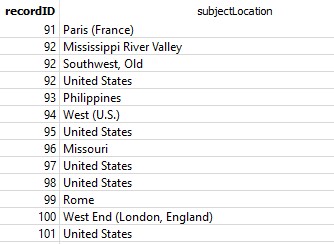
We have a mix of countries, cities, states, and descriptions of regions. The plan is to send each of these strings to a service that will geocode it, then return some associated data that we can use to make a map. We’ll use the Python package geopy, which provides access to several different geocoding service APIs (see A Practical Guide to Geopy). Let’s consider three different services:
| Service | API key required? | Query limits |
|---|---|---|
| Bing Map API | Yes | see documentation |
| Google Maps Geocoding | Yes | 2500 / day |
| Nominatim (Open Street Map) | No | 1 / second |
After parsing all 4.4 GB (compressed) of XML records, we end up with over 2.6 million location strings. Clearly the query limits are going to be a big factor in deciding which geocoding service to use, and we’ll need to reduce the number of queries sent as much as we can. Restricting to unique strings we end up with 131,170. We can reduce this further by using the tool OpenRefine to identify and cluster similar strings. This groups together similar strings and assigns a single value to each. We end up with 123,008 strings that we will need to geocode. We could manually check the data and eliminate some rows that don’t necessarily make sense for our project (“Solar system” for example), but I’ll just leave them in and consider whatever latitude and longitude is returned to be acceptable noise.
Caching Geocoded Data
Bing had the most generous free usage limits (~50,000 / day) at the time I was doing this geocoding. Even so, it’s fairly critical to create a cache of returned data from geocoding queries. Repeatedly sending the same queries to a geocoding service during development could get you blocked from that service. We may also decide in the future to pull some other elements out of the query return, which would be unavailable if we just saved the latitude and longitude and threw out the rest.
The strategy here is to create another SQLite table to store the query terms and results. Query results will be complicated nested dictionary structures. To cache this in our SQL database, we will have to “flatten” it using the Python package pickle. An excellent example of the entire caching process can be found in the answers to this question on stackoverflow.
Point vs. Country data
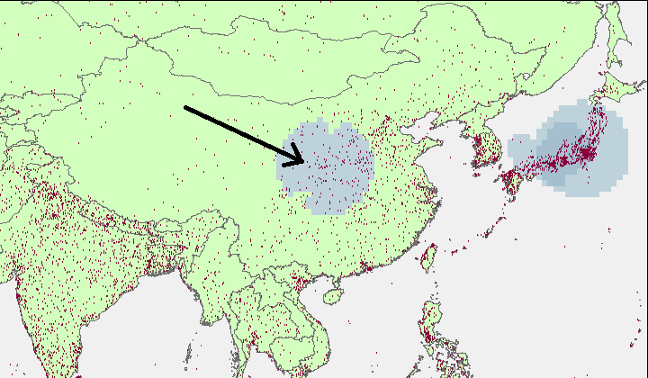
Let’s consider two possible formats that could be associated with each string: latitude / longitude points, or country codes. Geocoding services should always return a longitude and latitude point for a queried string, but they may not always identify a country code. However, the lat/long point returned for a string like “United States” will fall in the center of the country, and since “United States” is likely to be by far the most common string in the subject location field, plotting longitude and latitude points may incorrectly make Missouri look like the subject of way more writing than the rest of the country. Making a simple point density map illustrates how many points are mapped to the central point of China:
 [Download the point data]
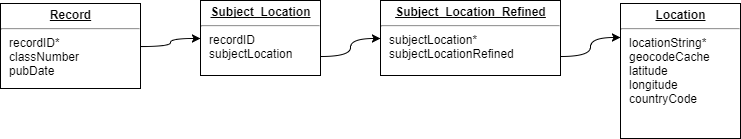
For this reason, we’ll want to just associate each record with a country. We can turn our longitude and latitude points into country codes pretty simply – by loading them in ArcGIS (or your favorite open source GIS) and spatially joining each point with the country it lies in. For this I used Natural Earth country boundaries. Great, now for each parsed subject location string we should have a refined string, a cached geocoded object, a longitude, a latitude, and an ISO country code. Here’s our database structure:
Joining these tables and summarizing by pubDate and countryCode, we have the following spreadsheet ready for a D3 visualization:
Finally, since we'll want to animate trends in changes in the number of book records per country over time, we want to make sure that countries don't flicker too much with year to year variances. To do this, I created another copy of this spreadsheet with new columns that simply take the sum of counts across three and five year windows respectively.